17 💻 PCA

17.1 Principal Components Analysis

We will use the following packages ‘FactoMineR’, ‘factoextra’, ‘ISRL2’

17.1.1 PCA using ‘FactoMineR’, ‘factoextra’

#> Loading required package: ggplot2
#> Welcome! Want to learn more? See two factoextra-related books at https://goo.gl/ve3WBa

17.1.2 Exercise 1 : read the data

#>    Var1 Var2
#> i1    2    2
#> i2    1   -1
#> i3   -1    1
#> i4   -2   -2

Covariance matrix

mean(X[,1]) # mean of Var1
#> [1] 0
mean(X[,2]) # mean of Var2
#> [1] 0

##variance and inertia 
S=var(X)*(3/4)  # the constant (n-1)/n is have the variance-covariance matrix used in the lecture
S
#>      Var1 Var2
#> Var1  2.5  1.5
#> Var2  1.5  2.5
#inertia
Inertia=sum(diag(S))
Inertia
#> [1] 5
## eigen-analysis
eigen(S) # gives the eigen-values and eigen-vectors
#> eigen() decomposition
#> $values
#> [1] 4 1
#> 
#> $vectors
#>           [,1]       [,2]
#> [1,] 0.7071068 -0.7071068
#> [2,] 0.7071068  0.7071068

Eigen-analysis on the correlation matrix

R=cor(X)
eigenan=eigen(R) ##eigen analysis of R
eigenan
#> eigen() decomposition
#> $values
#> [1] 1.6 0.4
#> 
#> $vectors
#>           [,1]       [,2]
#> [1,] 0.7071068 -0.7071068
#> [2,] 0.7071068  0.7071068
sum(eigenan$values)
#> [1] 2
#Inertia is p=2

#normalized the data
Z=scale(X)
var(Z) ## is teh correlation matrix 
#>      Var1 Var2
#> Var1  1.0  0.6
#> Var2  0.6  1.0

17.1.3 PCA function

PCA with the covariance matrix (using only centered data). For PCA on the correlation matrix (normed PCA), use scale.unit = TRUE (default option).

Correlation between two variables $X_{1}$ , $X_{2}$

$ρ = \frac{c o v (X_{1}, X_{2})}{σ_{X_{1}} σ_{X_{2}}}$ where $c o v (X_{1}, X_{2})$ is the covariance, $σ_{X_{1}} = \sqrt{V a r (X_{1})}$ is the standard deviation of $X_{1}$ .

Eigen-analysis on the covariance matrix (‘scale.unit=FALSE’)

#> **Results for the Principal Component Analysis (PCA)**
#> The analysis was performed on 4 individuals, described by 2 variables
#> *The results are available in the following objects:
#> 
#>    name               description                          
#> 1  "$eig"             "eigenvalues"                        
#> 2  "$var"             "results for the variables"          
#> 3  "$var$coord"       "coord. for the variables"           
#> 4  "$var$cor"         "correlations variables - dimensions"
#> 5  "$var$cos2"        "cos2 for the variables"             
#> 6  "$var$contrib"     "contributions of the variables"     
#> 7  "$ind"             "results for the individuals"        
#> 8  "$ind$coord"       "coord. for the individuals"         
#> 9  "$ind$cos2"        "cos2 for the individuals"           
#> 10 "$ind$contrib"     "contributions of the individuals"   
#> 11 "$call"            "summary statistics"                 
#> 12 "$call$centre"     "mean of the variables"              
#> 13 "$call$ecart.type" "standard error of the variables"    
#> 14 "$call$row.w"      "weights for the individuals"        
#> 15 "$call$col.w"      "weights for the variables"

17.1.4 Eigen-values

We have $p = 2 = m i n (n - 1, p) = m i n (3, 2)$ eigen-values, 4 and 1, $I n e r t i a = 4 + 1 = 4$ is the sum of the variances of the variables.

#>        eigenvalue percentage of variance
#> comp 1          4                     80
#> comp 2          1                     20
#>        cumulative percentage of variance
#> comp 1                                80
#> comp 2                               100

17.1.5 The variables

#> $coord
#>         Dim.1      Dim.2
#> Var1 1.414214 -0.7071068
#> Var2 1.414214  0.7071068
#> 
#> $cor
#>          Dim.1      Dim.2
#> Var1 0.8944272 -0.4472136
#> Var2 0.8944272  0.4472136
#> 
#> $cos2
#>      Dim.1 Dim.2
#> Var1   0.8   0.2
#> Var2   0.8   0.2
#> 
#> $contrib
#>      Dim.1 Dim.2
#> Var1    50    50
#> Var2    50    50

17.1.6 The inviduals

#> $coord
#>                         Dim.1                       Dim.2
#> i1  2.82842712474619073503845 -0.000000000000000006357668
#> i2  0.00000000000000001271534 -1.414213562373095367519227
#> i3 -0.00000000000000040992080  1.414213562373094923430017
#> i4 -2.82842712474619029094924  0.000000000000000204960400
#> 
#> $cos2
#>                                          Dim.1
#> i1 1.00000000000000044408920985006261616945267
#> i2 0.00000000000000000000000000000000008083988
#> i3 0.00000000000000000000000000000008401753104
#> i4 1.00000000000000022204460492503130808472633
#>                                           Dim.2
#> i1 0.000000000000000000000000000000000005052492
#> i2 1.000000000000000444089209850062616169452667
#> i3 0.999999999999999777955395074968691915273666
#> i4 0.000000000000000000000000000000005251095690
#> 
#> $contrib
#>                                         Dim.1
#> i1 50.000000000000021316282072803005576133728
#> i2  0.000000000000000000000000000000001010498
#> i3  0.000000000000000000000000000001050219138
#> i4 50.000000000000014210854715202003717422485
#>                                         Dim.2
#> i1  0.000000000000000000000000000000001010498
#> i2 50.000000000000021316282072803005576133728
#> i3 49.999999999999985789145284797996282577515
#> i4  0.000000000000000000000000000001050219138
#> 
#> $dist
#>       i1       i2       i3       i4 
#> 2.828427 1.414214 1.414214 2.828427

17.1.7 Another example

A=matrix(c(9,12,10,15,9,10,5,10,8,11,13,14,11,13,8,3,15,10),nrow=6, byrow=TRUE)
A
#>      [,1] [,2] [,3]
#> [1,]    9   12   10
#> [2,]   15    9   10
#> [3,]    5   10    8
#> [4,]   11   13   14
#> [5,]   11   13    8
#> [6,]    3   15   10
Nframe=as.data.frame(A)
m1=c("Alex", "Bea", "Claudio","Damien", "Emilie", "Fran")
m2=c("Biostatistics", "Economics", "English")
row.names(A)=m1
colnames(A)=m2
head(A)
#>         Biostatistics Economics English
#> Alex                9        12      10
#> Bea                15         9      10
#> Claudio             5        10       8
#> Damien             11        13      14
#> Emilie             11        13       8
#> Fran                3        15      10

17.1.8 PCA on the correlation matrix

#> **Results for the Principal Component Analysis (PCA)**
#> The analysis was performed on 6 individuals, described by 3 variables
#> *The results are available in the following objects:
#> 
#>    name               description                          
#> 1  "$eig"             "eigenvalues"                        
#> 2  "$var"             "results for the variables"          
#> 3  "$var$coord"       "coord. for the variables"           
#> 4  "$var$cor"         "correlations variables - dimensions"
#> 5  "$var$cos2"        "cos2 for the variables"             
#> 6  "$var$contrib"     "contributions of the variables"     
#> 7  "$ind"             "results for the individuals"        
#> 8  "$ind$coord"       "coord. for the individuals"         
#> 9  "$ind$cos2"        "cos2 for the individuals"           
#> 10 "$ind$contrib"     "contributions of the individuals"   
#> 11 "$call"            "summary statistics"                 
#> 12 "$call$centre"     "mean of the variables"              
#> 13 "$call$ecart.type" "standard error of the variables"    
#> 14 "$call$row.w"      "weights for the individuals"        
#> 15 "$call$col.w"      "weights for the variables"

17.1.9 Eigen-values

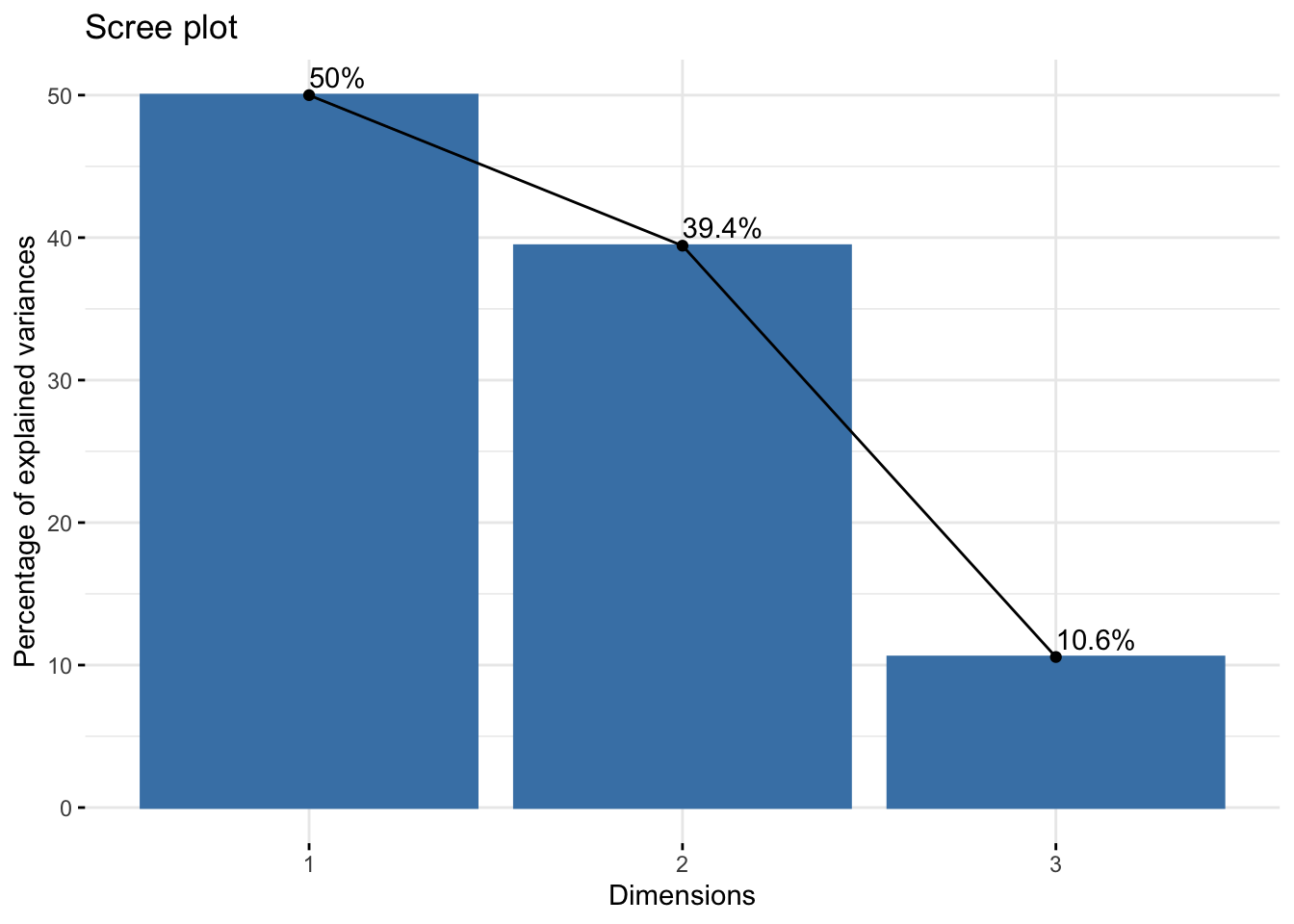
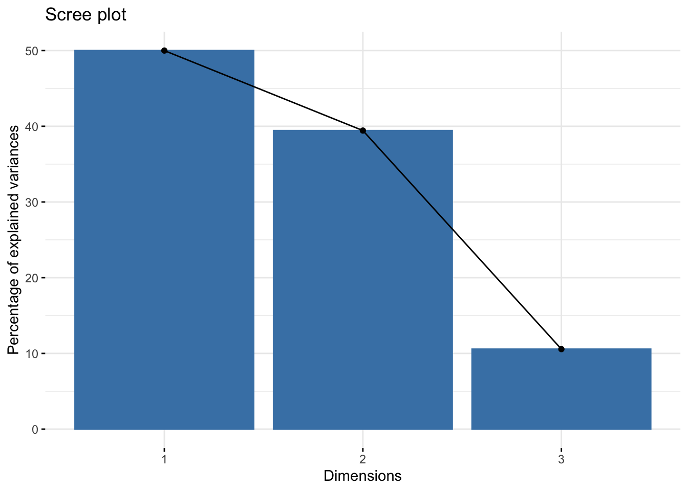
#>        eigenvalue percentage of variance
#> comp 1  1.5000000               50.00000
#> comp 2  1.1830127               39.43376
#> comp 3  0.3169873               10.56624
#>        cumulative percentage of variance
#> comp 1                          50.00000
#> comp 2                          89.43376
#> comp 3                         100.00000
#>       eigenvalue variance.percent
#> Dim.1  1.5000000         50.00000
#> Dim.2  1.1830127         39.43376
#> Dim.3  0.3169873         10.56624
#>       cumulative.variance.percent
#> Dim.1                    50.00000
#> Dim.2                    89.43376
#> Dim.3                   100.00000

Kaiser rule suggests $q = 2$ components because the eigen-value mean is 1 (with 89% of explained variance). The rule of Thumb gives $q = 2$ because the first 2 dimensions explain 89% of the variance/inertia.

17.1.10 Variables

#> Principal Component Analysis Results for variables
#>  ===================================================
#>   Name      
#> 1 "$coord"  
#> 2 "$cor"    
#> 3 "$cos2"   
#> 4 "$contrib"
#>   Description                                    
#> 1 "Coordinates for the variables"                
#> 2 "Correlations between variables and dimensions"
#> 3 "Cos2 for the variables"                       
#> 4 "contributions of the variables"

17.1.11 Correlations of variables and components/dimensions

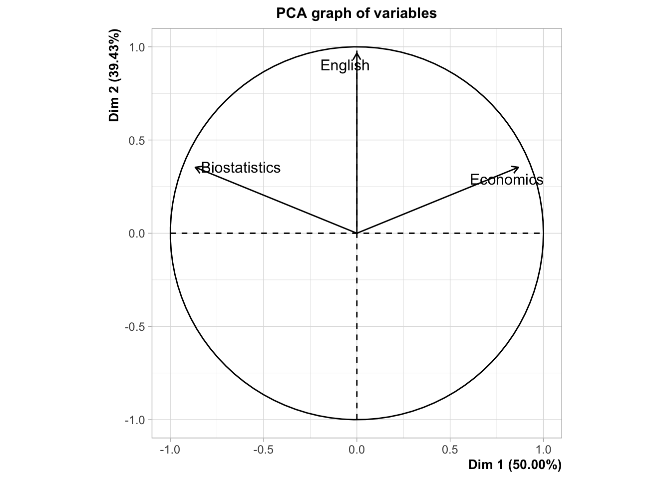
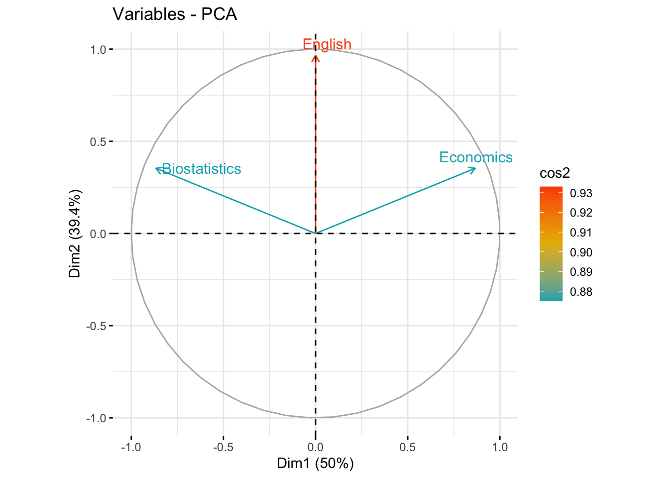
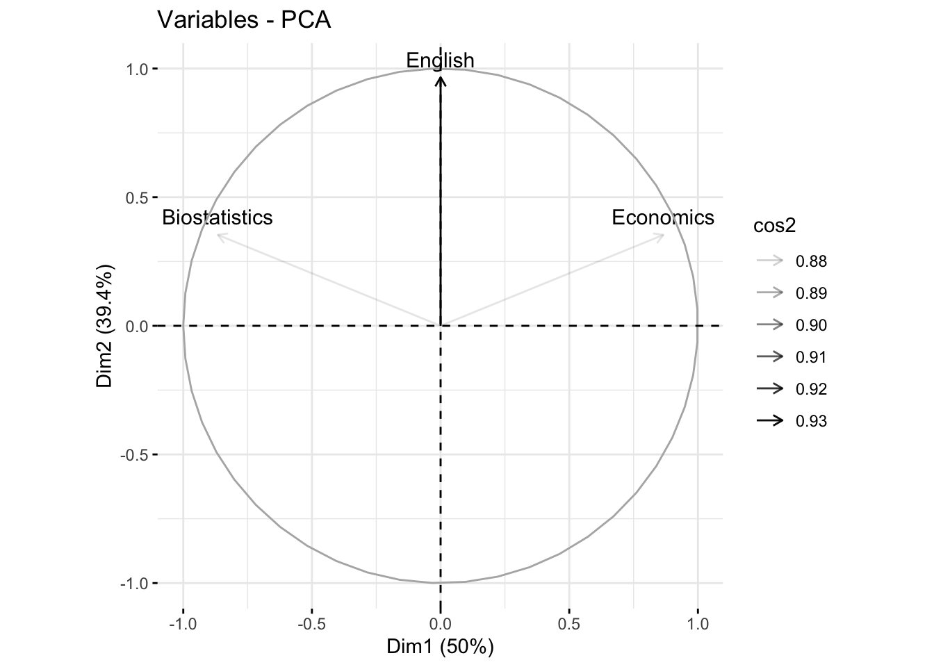
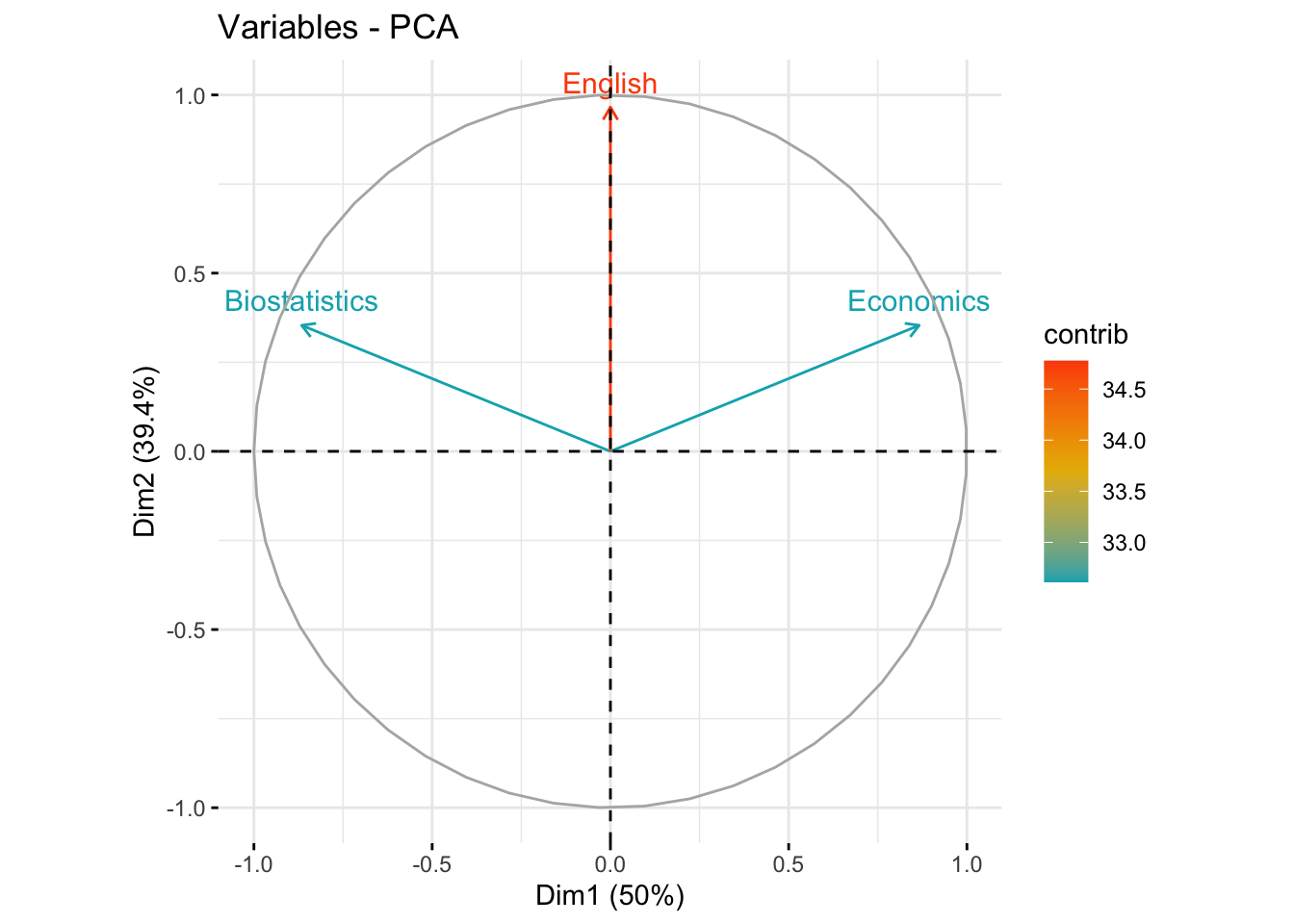
#>                                  Dim.1     Dim.2      Dim.3
#> Biostatistics -0.866025403784438041477 0.3535534  0.3535534
#> Economics      0.866025403784439151700 0.3535534  0.3535534
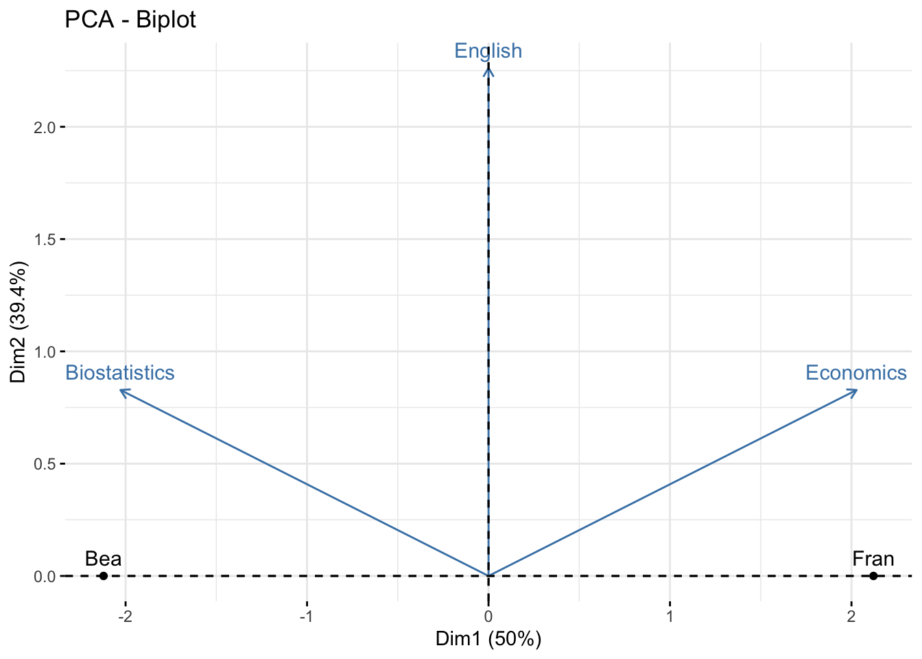
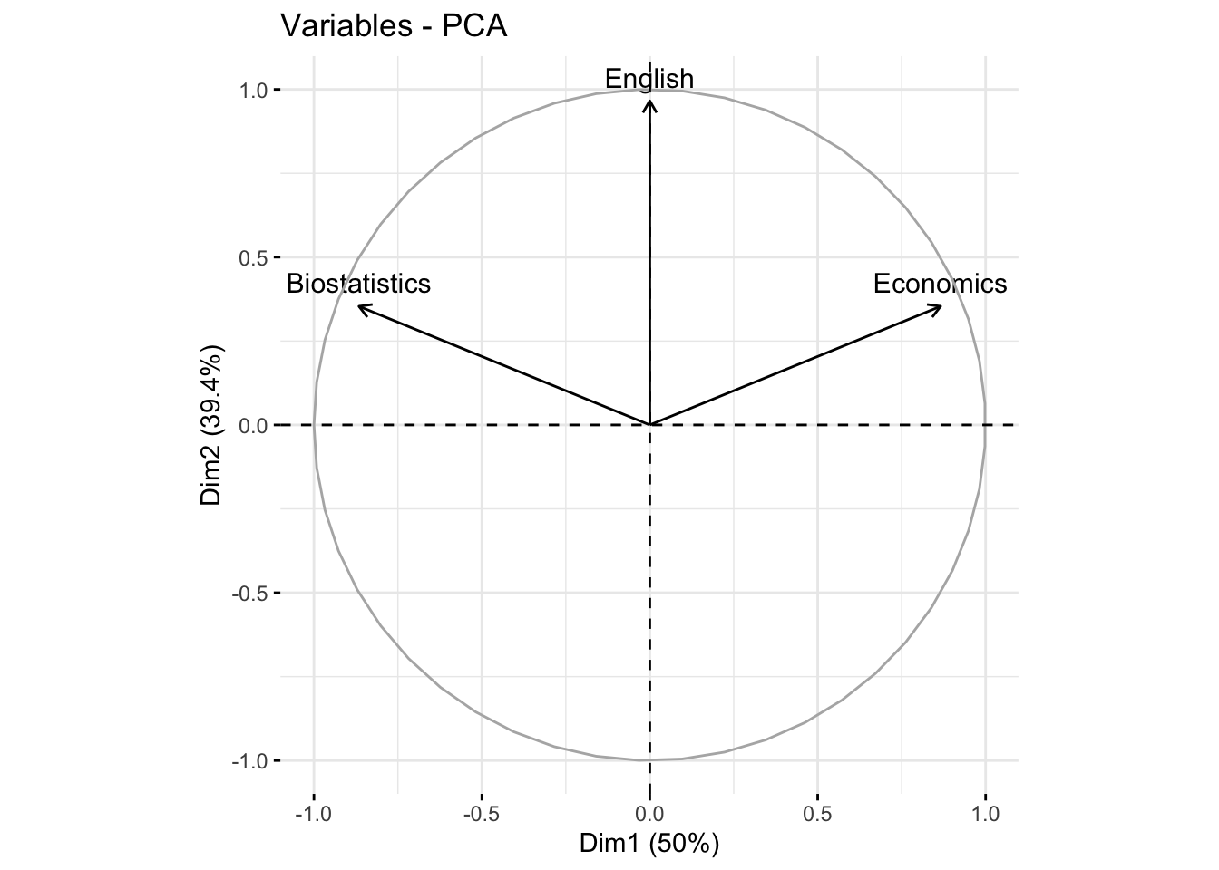
#> English        0.000000000000001047394 0.9659258 -0.2588190

The first axis is correlated with Biostatistics (+0.86) and Economics (-0.86). The second axis is correlated to English (0.96).

The two components (or dimensions) are correlated with at least one variable. Then $q = 2$ may be considered to reduce the dimension ( $p = 3$ ).

17.1.12 Coordinates of variables

#>                                  Dim.1     Dim.2      Dim.3
#> Biostatistics -0.866025403784438041477 0.3535534  0.3535534
#> Economics      0.866025403784439040678 0.3535534  0.3535534
#> English        0.000000000000001047394 0.9659258 -0.2588190

17.1.13 Quality of representation of variables

#>                                                Dim.1
#> Biostatistics 0.749999999999999000799277837359113619
#> Economics     0.750000000000000888178419700125232339
#> English       0.000000000000000000000000000001097035
#>                   Dim.2     Dim.3
#> Biostatistics 0.1250000 0.1250000
#> Economics     0.1250000 0.1250000
#> English       0.9330127 0.0669873

Biostatistics and Economics are well represented in the first dimension (75%), while English is very well represented in the second axis (93%). In the first plane (Dim.1 and Dim.2) Biostatistics and Economics are well represented (75%+12.5%=87.5%), English is very represented in the first plane (93%+0%=93%)

17.1.14 Contributions of variables

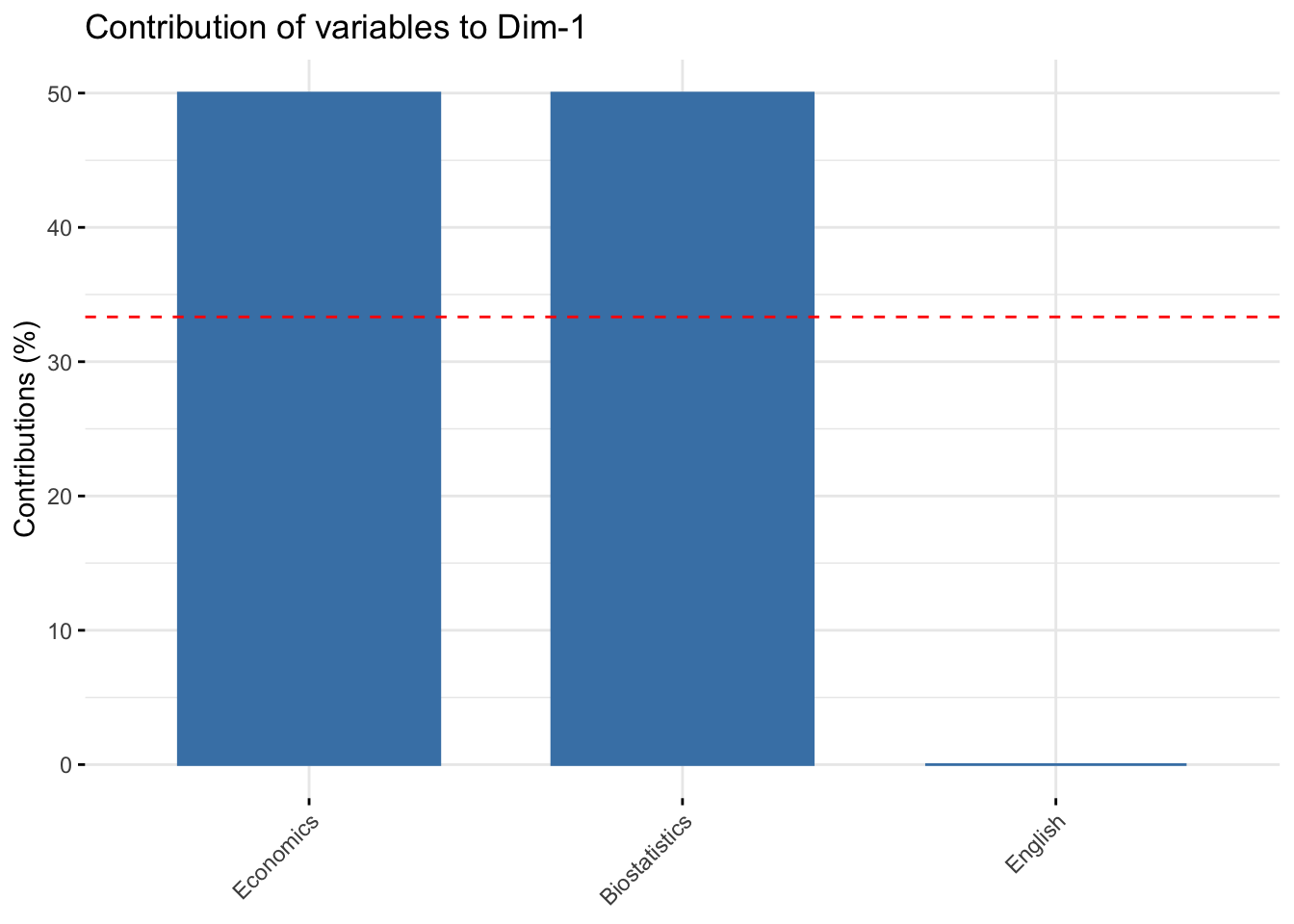
#>                                                Dim.1
#> Biostatistics 49.99999999999993605115378159098327160
#> Economics     50.00000000000005684341886080801486969
#> English        0.00000000000000000000000000007313567
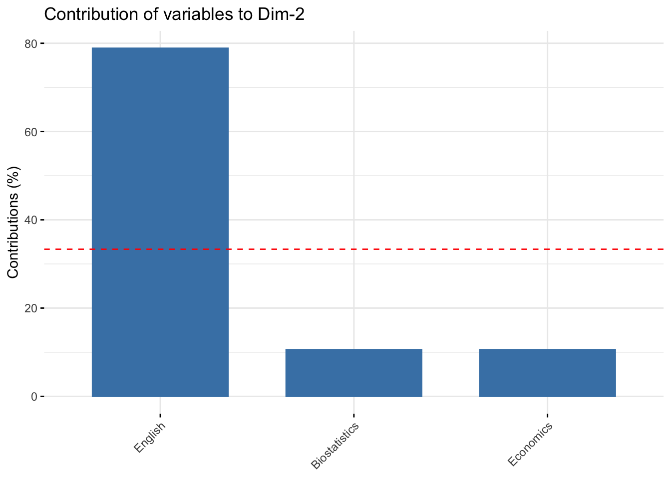
#>                  Dim.2    Dim.3
#> Biostatistics 10.56624 39.43376
#> Economics     10.56624 39.43376
#> English       78.86751 21.13249

Biostatistics and Economics contribute to the construction of the first dimension (50%), while English contribute highy to the construction of the second axis (78.8%). In the first plane (Dim.1 and Dim.2) the contribution of Biostatistics and Economics is 50%+10.5%=65.5%, that of English is 78.8%.

Description of the first dimension

#> 
#> Link between the variable and the continuous variables (R-square)
#> =================================================================================
#>               correlation    p.value
#> Economics       0.8660254 0.02572142
#> Biostatistics  -0.8660254 0.02572142

17.1.15 Contributions of first two variables

#>               Dim.1    Dim.2    Dim.3
#> Biostatistics    50 10.56624 39.43376
#> Economics        50 10.56624 39.43376

17.1.16 Representation of variables

17.1.17 With the quality of representation

17.1.18 With the quality of representation

17.1.19 Variables with quality of representation larger than 0.6

17.1.20 With contribution

17.1.21 Variables and individus with largest quality of representation

17.1.22 The individuals

#> Principal Component Analysis Results for individuals
#>  ===================================================
#>   Name       Description                       
#> 1 "$coord"   "Coordinates for the individuals" 
#> 2 "$cos2"    "Cos2 for the individuals"        
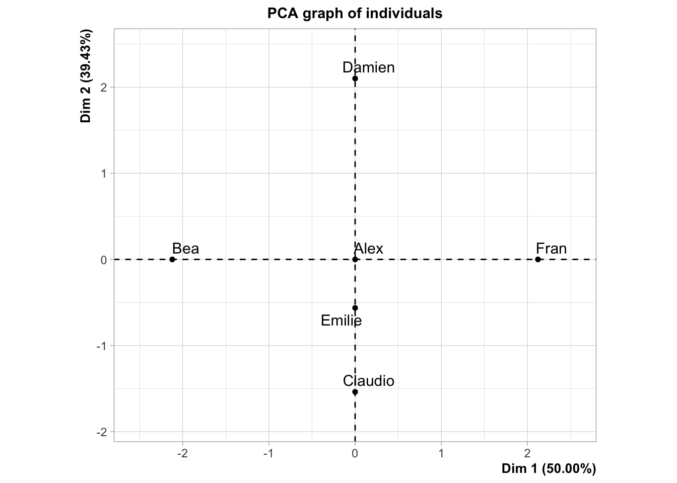
#> 3 "$contrib" "contributions of the individuals"

17.1.23 Individuals: coordinates

#>                             Dim.1                    Dim.2
#> Alex     0.0000000000000002653034 -0.000000000000000941663
#> Bea     -2.1213203435596423851450  0.000000000000001237395
#> Claudio -0.0000000000000022171779 -1.538189001320852344890
#> Damien   0.0000000000000026937746  2.101205251626097503248
#> Emilie   0.0000000000000001895371 -0.563016250305248155961
#> Fran     2.1213203435596428292342 -0.000000000000002975084
#>                              Dim.3
#> Alex    -0.00000000000000007994654
#> Bea      0.00000000000000015526499
#> Claudio -0.79622521701812609684623
#> Damien  -0.29143865656241157990891
#> Emilie   1.08766387358053817635550
#> Fran     0.00000000000000002468473
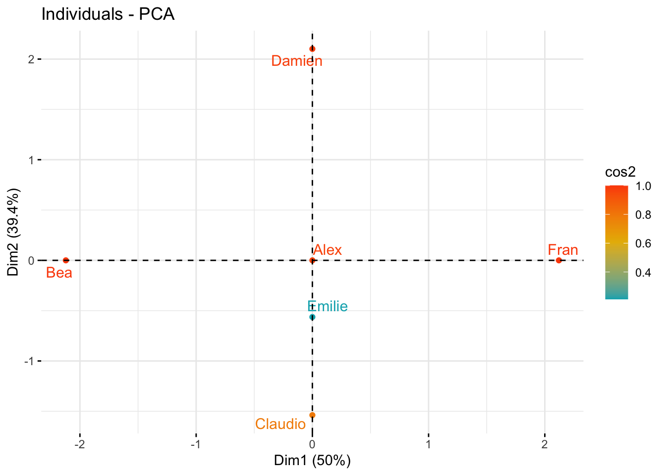
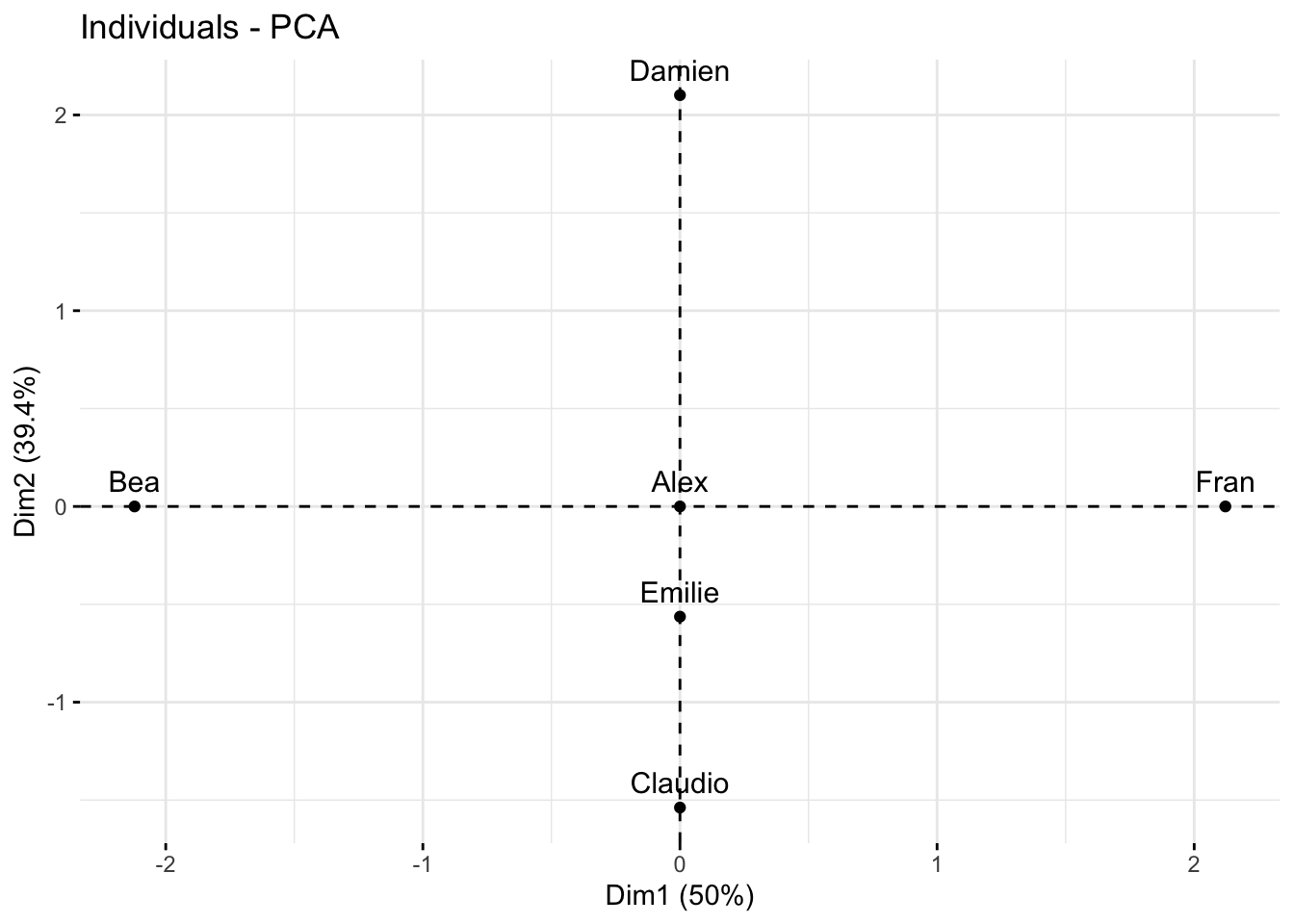
#>                             Dim.1                    Dim.2
#> Alex     0.0000000000000002653034 -0.000000000000000941663
#> Bea     -2.1213203435596423851450  0.000000000000001237395
#> Claudio -0.0000000000000022171779 -1.538189001320852344890
#> Damien   0.0000000000000026937746  2.101205251626097503248
#> Emilie   0.0000000000000001895371 -0.563016250305248155961
#> Fran     2.1213203435596428292342 -0.000000000000002975084
#>                              Dim.3
#> Alex    -0.00000000000000007994654
#> Bea      0.00000000000000015526499
#> Claudio -0.79622521701812609684623
#> Damien  -0.29143865656241157990891
#> Emilie   1.08766387358053817635550
#> Fran     0.00000000000000002468473

17.1.24 Quality of representation

#>                                            Dim.1
#> Alex    0.07137976857538211317155685264879139140
#> Bea     1.00000000000000022204460492503130808473
#> Claudio 0.00000000000000000000000000000163862588
#> Damien  0.00000000000000000000000000000161253810
#> Emilie  0.00000000000000000000000000000002394954
#> Fran    0.99999999999999977795539507496869191527
#>                                           Dim.2
#> Alex    0.8992501752497785716400358069222420454
#> Bea     0.0000000000000000000000000000003402549
#> Claudio 0.7886751345948129765517364830884616822
#> Damien  0.9811252243246878501636842884181533009
#> Emilie  0.2113248654051877173376539076343760826
#> Fran    0.0000000000000000000000000000019669168
#>                                             Dim.3
#> Alex    0.006481699860810073883510273873298501712
#> Bea     0.000000000000000000000000000000005357159
#> Claudio 0.211324865405187134470565979427192360163
#> Damien  0.018874775675311854933324795524640649091
#> Emilie  0.788675134594813309618643870635423809290
#> Fran    0.000000000000000000000000000000000135408

17.1.25 Contributions

#>                                            Dim.1
#> Alex     0.0000000000000000000000000000007820654
#> Bea     50.0000000000000000000000000000000000000
#> Claudio  0.0000000000000000000000000000546208628
#> Damien   0.0000000000000000000000000000806269052
#> Emilie   0.0000000000000000000000000000003991590
#> Fran    50.0000000000000213162820728030055761337
#>                                          Dim.2
#> Alex     0.00000000000000000000000000001249253
#> Bea      0.00000000000000000000000000002157130
#> Claudio 33.33333333333337833437326480634510517
#> Damien  62.20084679281458051036679535172879696
#> Emilie   4.46581987385206335972043234505690634
#> Fran     0.00000000000000000000000000012469753
#>                                             Dim.3
#> Alex     0.00000000000000000000000000000033605182
#> Bea      0.00000000000000000000000000000126751744
#> Claudio 33.33333333333333570180911920033395290375
#> Damien   4.46581987385203582618942164117470383644
#> Emilie  62.20084679281465867006772896274924278259
#> Fran     0.00000000000000000000000000000003203788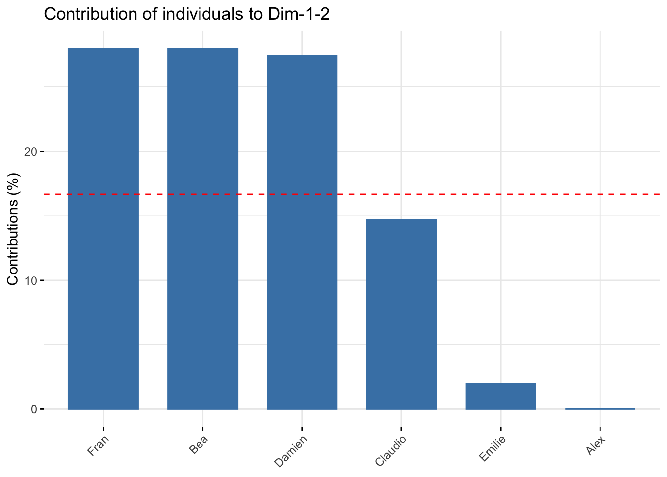

17.1.26 Contributions on the first two axes

17.1.27 Representation of individuals with respect to quality of projection

17.1.28 Save the figures in pdf

17.1.29 Save in png

17.1.30 Another saving

#> file saved to PCA.pdf
#> file saved to PCA.pdf
#> [1] "PCA%03d.png"
#> file saved to PCA%03d.png

17.1.31 Export the results in txt fimes

17.2 PCA with prcomp function of the base `R` package

Here we perform PCA on the USArrests, the rows of the data set contain the 50 states, in alphabetical order.

?USArrests will give details on the dataframe View(USArrests) to see the whole dataframe

#>  [1] "Alabama"        "Alaska"         "Arizona"       
#>  [4] "Arkansas"       "California"     "Colorado"      
#>  [7] "Connecticut"    "Delaware"       "Florida"       
#> [10] "Georgia"        "Hawaii"         "Idaho"         
#> [13] "Illinois"       "Indiana"        "Iowa"          
#> [16] "Kansas"         "Kentucky"       "Louisiana"     
#> [19] "Maine"          "Maryland"       "Massachusetts" 
#> [22] "Michigan"       "Minnesota"      "Mississippi"   
#> [25] "Missouri"       "Montana"        "Nebraska"      
#> [28] "Nevada"         "New Hampshire"  "New Jersey"    
#> [31] "New Mexico"     "New York"       "North Carolina"
#> [34] "North Dakota"   "Ohio"           "Oklahoma"      
#> [37] "Oregon"         "Pennsylvania"   "Rhode Island"  
#> [40] "South Carolina" "South Dakota"   "Tennessee"     
#> [43] "Texas"          "Utah"           "Vermont"       
#> [46] "Virginia"       "Washington"     "West Virginia" 
#> [49] "Wisconsin"      "Wyoming"

The columns of the data set contain four variables:

-Murder: Murder arrests (per 100,000) -Assault: Assault arrests (per 100,000) -UrbanPop: Percent urban population -Rape: Rape arrests (per 100,000)

#> [1] "Murder"   "Assault"  "UrbanPop" "Rape"

Notice that the variables have vastly different means (of variables in columns), with the apply() function. ‘apply(USArrests, 2, mean)’ permits to calculate the means of each column, the option ‘1’ will do the calculation by row

#>   Murder  Assault UrbanPop     Rape 
#>    7.788  170.760   65.540   21.232

There are on average three times as many rapes as murders, and more than eight times as many assaults as rapes. Let us also examine the variances of the variables

#>     Murder    Assault   UrbanPop       Rape 
#>   18.97047 6945.16571  209.51878   87.72916

The variables have very different variances: the UrbanPop variable measuring the percentage of the population in each state living in an urban area, is not a comparable number to the number of rapes in each state per 100,000 individuals. If we do not scale the variables before performing PCA, then most of the principal components that we observed would be driven by the Assault variable, since it has the largest mean and variance. Here, it is important to standardize the variables to have mean zero and standard deviation one before performing PCA.

The option scale = TRUE, does a scaling of the variables to have standard deviation one.

#> [1] "sdev"     "rotation" "center"   "scale"    "x"

The center and scale components correspond to the means and standard deviations of the variables that were used for scaling prior to implementing PCA.

#>   Murder  Assault UrbanPop     Rape 
#>    7.788  170.760   65.540   21.232
#>    Murder   Assault  UrbanPop      Rape 
#>  4.355510 83.337661 14.474763  9.366385

The rotation matrix provides the principal component loadings; each column of pr.out$rotation contains the corresponding principal component loading vector.

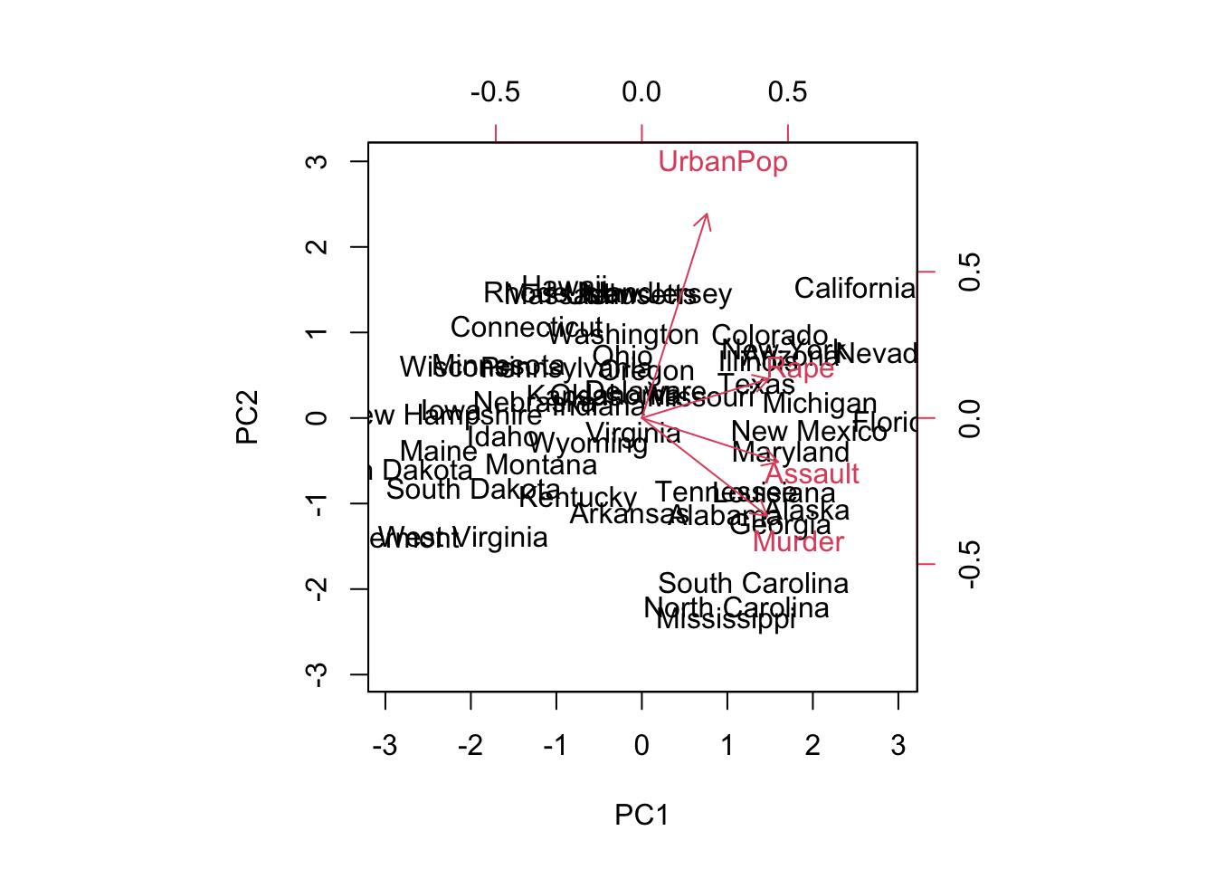
#>                 PC1        PC2        PC3         PC4
#> Murder   -0.5358995  0.4181809 -0.3412327  0.64922780
#> Assault  -0.5831836  0.1879856 -0.2681484 -0.74340748
#> UrbanPop -0.2781909 -0.8728062 -0.3780158  0.13387773
#> Rape     -0.5434321 -0.1673186  0.8177779  0.08902432

We see that there are four distinct principal components. This is to be expected because there are in general $min (n - 1, p)$ informative principal components in a data set with $n$ observations and $p$ variables.

Using the pr.out$x we have the $50 \times 4$ matrix x principal component score vectors. That is, the $k$ th column is the $k$ th principal component score vector.

#> [1] 50  4
#>                   PC1        PC2         PC3          PC4
#> Alabama    -0.9756604  1.1220012 -0.43980366  0.154696581
#> Alaska     -1.9305379  1.0624269  2.01950027 -0.434175454
#> Arizona    -1.7454429 -0.7384595  0.05423025 -0.826264240
#> Arkansas    0.1399989  1.1085423  0.11342217 -0.180973554
#> California -2.4986128 -1.5274267  0.59254100 -0.338559240
#> Colorado   -1.4993407 -0.9776297  1.08400162  0.001450164

We can plot the first two principal components as follows:

The scale = 0 argument to biplot() ensures that the arrows are scaled to represent the loadings; other values for scale give slightly different biplots with different interpretations.

The principal components are only unique up to a sign change, so we can reproduce the above figure by making a small changes:

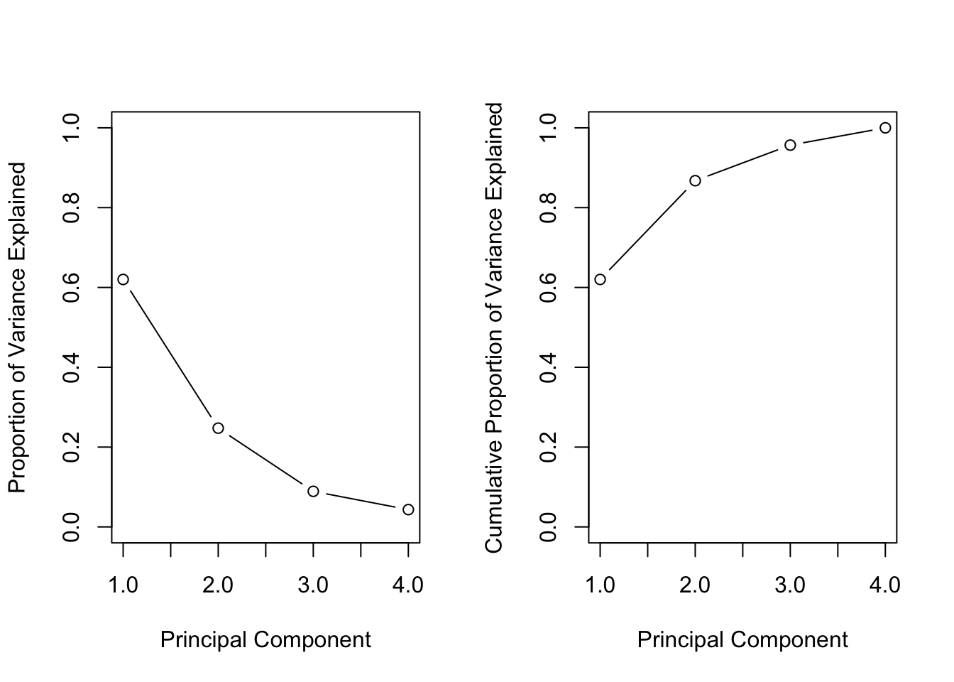
The standard deviation (square root of the corresponding eigen-value) of each principal component is as follows:

#> [1] 1.5748783 0.9948694 0.5971291 0.4164494

The variance explained by each principal component (corresponding eigen-value) is obtained by squaring these:

#> [1] 2.4802416 0.9897652 0.3565632 0.1734301

Compute the proportion of variance explained by each principal component as follows

#> [1] 0.62006039 0.24744129 0.08914080 0.04335752

We see that the first principal component explains $62.0 %$ of the variance in the data, the next principal component explains $24.7 %$ of the variance. Plot the PVE (Proportion of Variance Explained) explained by each component, and the cumulative PVE, as follows:

The function cumsum() computes the cumulative sum of the elements of a numeric vector.

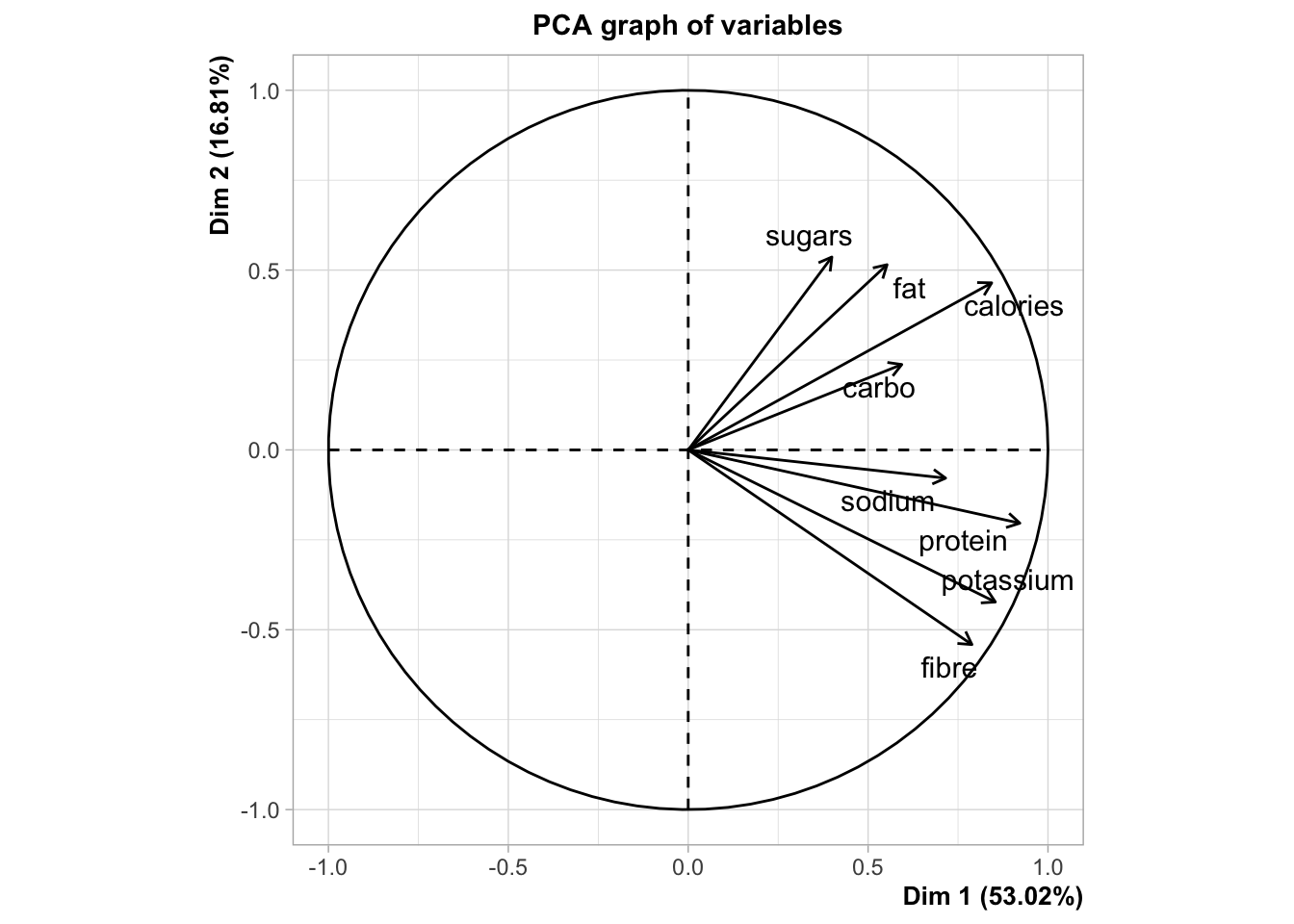
17.3 Exercise 1: Nutritional and Marketing Information on US Cereals

Consider the UScereal data (65 rows and 11 columns, package ‘MASS’) from the 1993 ASA Statistical Graphics Exposition and taken from the mandatory F&DA food label. The data have been normalized here to a portion of one American cup.

#> 
#> Attaching package: 'MASS'
#> The following object is masked from 'package:dplyr':
#> 
#>     select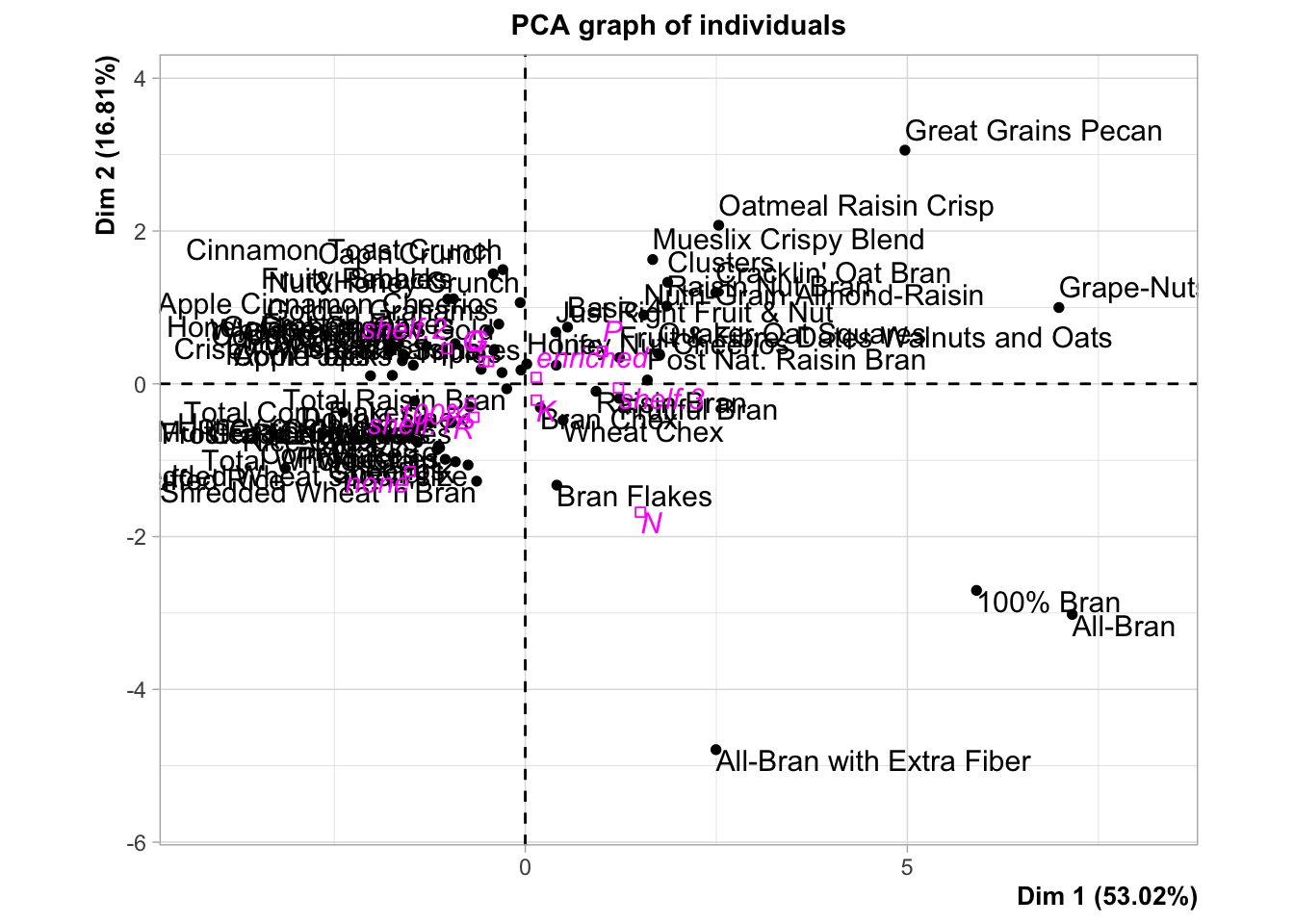

#> Error in PCA(UScereal): 
#> The following variables are not quantitative:  mfr
#> The following variables are not quantitative:  vitamins

17.4 Exercise 2

Consider the NCI cancer cell line microarray data, which consists of $6,830$ gene expression measurements on $64$ cancer cell lines.

#> 
#> Attaching package: 'ISLR2'
#> The following object is masked from 'package:MASS':
#> 
#>     Boston

Each cell line is labeled with a cancer type, given in nci.labs.

17.4.1 Exercise 3: Wine Quality Analysis

Consider the wine dataset available in the gclus package, which contains chemical analyses of wines grown in the same region in Italy but derived from three different cultivars. The dataset has 13 variables and over 170 observations.

library(gclus)
#> Loading required package: cluster
data(wine)

17.4.1.1 Tasks:

(a) Perform PCA on the wine dataset. Remember to standardize the variables if necessary, as they might be on different scales.
```
# Example code snippet
library(FactoMineR)
res.pca.wine <- PCA(wine, scale.unit = TRUE, graph = FALSE)
```
(b) Interpret the PCA results. Focus on understanding which chemical properties contribute most to the variance in the dataset and if the wines cluster by cultivar.

17.4.2 Exercise 4: Boston Housing Data Analysis

Consider the Boston dataset from the MASS package, which contains information collected by the U.S Census Service concerning housing in the area of Boston Mass. It has 506 rows and 14 columns.

library(MASS)
data(Boston)

17.4.2.1 Tasks:

(a) Conduct PCA on the Boston housing dataset. Before performing PCA, assess which variables are most suitable for the analysis and preprocess the data accordingly.
```
# Example code snippet
library(FactoMineR)
res.pca.boston <- PCA(Boston, scale.unit = TRUE, graph = FALSE)
```
(b) Interpret the results of the PCA. Look for patterns that might indicate relationships between different aspects of the housing data, such as crime rates, property tax, and median value of owner-occupied homes.

17.4.3 Notes for Solving:

Data Preprocessing: Before performing PCA, it’s crucial to preprocess the data. This may include handling missing values, standardizing the data, and selecting relevant variables.
PCA Interpretation: When interpreting the results, focus on the eigenvalues, the proportion of variance explained by the principal components, and the loadings of the variables on the principal components.
Visualization: Use plots like scree plots, biplots, or individual component plots to aid in your interpretation, use packages that do that for you!
Contextual Understanding: Each dataset has its context. Understanding the domain can significantly help in interpreting the results meaningfully.

16 💻 Binary LogReg exer

18 💻 Poisson regr exer