21 💻 Regression Trees

Regression trees are a type of machine learning algorithm that can be used to predict the value of a target variable based on the values of other variables. The algorithm works by splitting the data into smaller and smaller subsets, each subset containing data points with similar values for the target variable. By doing this, the algorithm can build a tree-like structure that can be used to make predictions about the target variable.

The advantages of using regression trees include their ability to handle non-linear relationships between variables, their ability to handle large datasets, and their ability to provide interpretable results. The main disadvantage is that they tend to overfit the data, meaning they may not generalize well to unseen data.

If you are stuck either ask to the TA or team work! Collaboration is always key 👯‍♂️! As you may notice the functioning is pretty similar to hierarchical clsutering, so we will not spend too much time on that!

21.0.1 train and test splitting

For this methods generally you need to train and test split data. There are a number of ways to do that, we will cover 2: one with base::r (without importing any package), the other with importing $r s a m p \leq s$ `

library(rpart)
library(rpart.plot)  # plotting regression trees
library(rsample)
library(factoextra)
#> Loading required package: ggplot2
#> Welcome! Want to learn more? See two factoextra-related books at https://goo.gl/ve3WBa

Lets also see how clusters change wrt the number of $k$ s

set.seed(28)

scale_USArrests = scale(USArrests)

k2 <- kmeans(scale_USArrests, centers = 2, nstart = 25)
k3 <- kmeans(scale_USArrests, centers = 3, nstart = 25)
k4 <- kmeans(scale_USArrests, centers = 4, nstart = 25)
k5 <- kmeans(scale_USArrests, centers = 5, nstart = 25)

# plots to compare
p1 <- fviz_cluster(k2, geom = "point", data = scale_USArrests) + ggtitle("k = 2")
p2 <- fviz_cluster(k3, geom = "point",  data = scale_USArrests) + ggtitle("k = 3")
p3 <- fviz_cluster(k4, geom = "point",  data = scale_USArrests) + ggtitle("k = 4")
p4 <- fviz_cluster(k5, geom = "point",  data = scale_USArrests) + ggtitle("k = 5")

library(gridExtra)
#> 
#> Attaching package: 'gridExtra'
#> The following object is masked from 'package:dplyr':
#> 
#>     combine
grid.arrange(p1, p2, p3, p4, nrow = 2)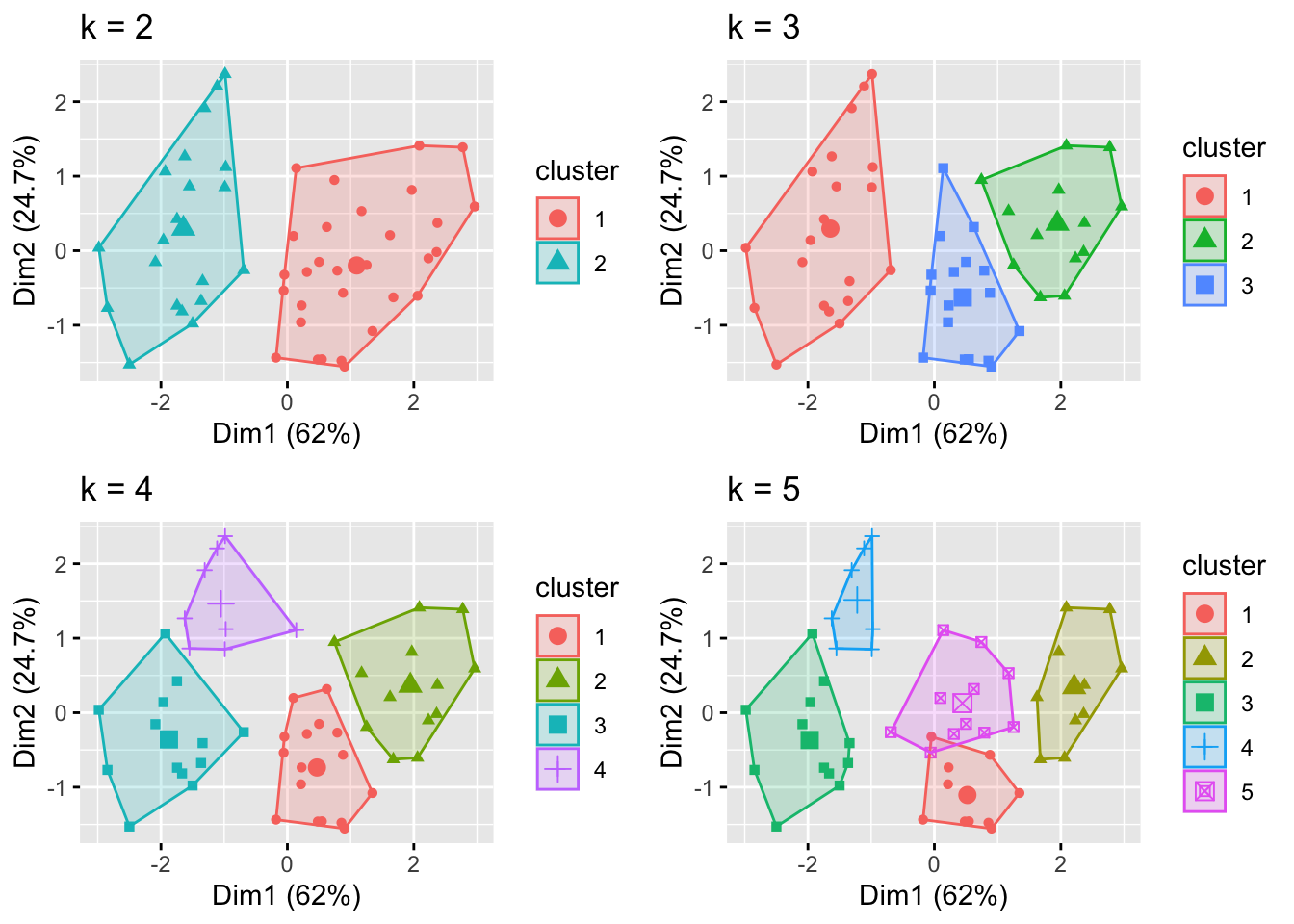

21.1 Exercises 👨‍💻

Exercise 20.1 Let’s have a look at an example in R using the Chatterjee-Price Attitude Data from the library(datasets) package. The dataset is a survey of clerical employees of a large financial organization. The data are aggregated from questionnaires of approximately 35 employees for each of 30 (randomly selected) departments. The numbers give the percent proportion of favourable responses to seven questions in each department. For more details, see ?attitude. We take a subset of the attitude dataset and consider only two variables in our K-Means clustering exercise i.e. privileges learning.

visualize privileges and learning in a scatterplot. Do you see any cluster?
apply algorithm kmeans on data with $k = 2$ and visualize results through the function fviz_cluster
now let’s try with $k = 3$ , by visual inspection , do you think it is better?

Remember how to use kmeans which is in base::R.

Answer to Question 20.1:

at first select variables from data:

library(dplyr)
selected_data = select(attitude, privileges, learning)
plot(selected_data,  pch =20, cex =2)

execute k-means algo:

set.seed(28)
km1 = kmeans(selected_data, k = 2, nstart=100)
fviz_cluster(km1, geom = "point", data = selected_data)

let’s try with k = 3

km2 = kmeans(selected_data, k =  3, nstart=100)
fviz_cluster(km2, geom = "point", data = selected_data)

21.2 bonus: elbow method ✨

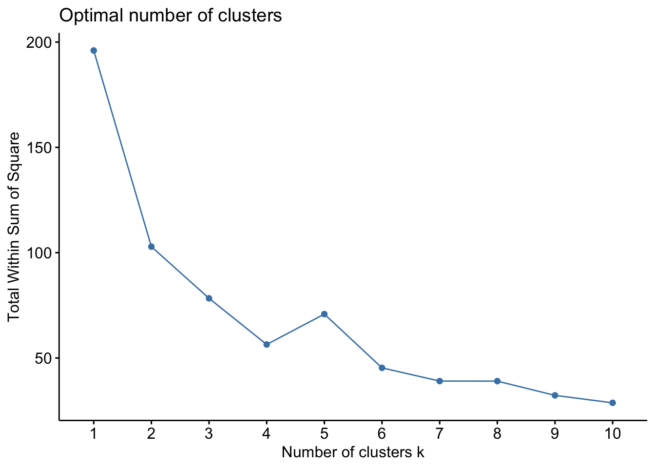
The main goal of cluster partitioning algorithms, such as k-means clustering, is to minimize the total intra-cluster variation, also known as the total within-cluster variation or total within-cluster sum of square.

minimize(_{k = 1}^{k}W(C_k)) $$ where $C_{k}$ is the $k^{t h}$ cluster and $W (C_{k})$ is the within-cluster variation. The total within-cluster sum of square (wss) measures the compactness of the clustering and we want it to be as small as possible. Thus, we can use the following algorithm to define the optimal clusters:

Compute clustering algorithm (e.g., k-means clustering) for different values of k. For instance, by varying k from 1 to 10 clusters
For each k, calculate the total within-cluster sum of square (wss)
Plot the curve of wss according to the number of clusters k.
The location of a bend (knee) in the plot is generally considered as an indicator of the appropriate number of clusters.

21.2.1 code implementation

Data is the same as beginning


fviz_nbclust(scale_USArrests, kmeans, method = "wss")

20 💻 K-Means Clustering

22 ⚡ course performance